
Welcome back to Nova Quant Lab. In earlier sessions we built our Python environment and a secure, real-time data bridge to the Binance API, so you can already ingest live market data and fire automated orders. But before I trusted Aurora Layer XQ — the EMA + RSI + Bollinger + ADX strategy I now run live on USDJPY 1H, with a publicly verified track record on myfxbook — with real capital, I had to cross the most treacherous part of quant development: backtesting.
The first time I crossed it, my backtest looked like a gold mine. My live account, when it finally went on, agreed only partway. This article is not another textbook list of biases you can find on a hundred other sites. It is the exact set of traps that made my backtest exaggerate, the live divergence that exposed them, and the validation discipline I built afterward — backed by the real numbers from both my four-year backtest and my live broker account, which you can audit yourself.
1. The Illusion of Profit: Why Raw Backtests Lie
The most humbling experience for a new quant is designing a system that prints a triple-digit return in a backtest, then watching it underperform the moment it goes live. This is almost never bad luck. It is a statistical artifact. When a backtest lies, it is usually committing one of three cardinal sins.
Trap 1: Overfitting (Curve Fitting)
Overfitting happens when you make a strategy so complex that it “fits” past price movements perfectly. Optimize across ten indicators, fifty micro-parameters, and exact time-of-day rules and you have not discovered a market truth — you have forced your code to memorize the past. Every parameter you add increases the degrees of freedom, making it exponentially more likely that your stellar result is random noise rather than a repeatable edge.
What works instead: keep the logic ruthlessly simple. A clean structural signal (a moving-average regime combined with a volatility and trend-strength filter) will usually beat a “Frankenstein” model in out-of-sample trading. If a strategy only shows a profit after microscopic parameter tweaking, the underlying edge is broken. When I tuned Aurora Layer XQ, I deliberately froze the indicator stack early and refused to add new inputs just because they nudged the equity curve upward on historical data.
Trap 2: Survivorship Bias
Test a stock algorithm only on today’s index leaders and you ignore every company that was delisted or went to zero during your test window. Your algorithm looks brilliant because it only ever traded survivors. The same trap exists in crypto: backtest from 2018 to 2026 on the coins that are still listed and you have quietly excluded LUNA, FTT, and the rest of the graveyard.
What works instead: use point-in-time datasets that include the failures. Forex is more forgiving here — a major pair like USDJPY does not get delisted — but the principle still applies to the regime. My USDJPY backtest spans 2022 through 2025 on purpose, because that window contains the violent yen depreciation, the Bank of Japan interventions, and the quiet ranging months. Only by testing across all of those regimes can you validate that a strategy survives more than one type of market.
Trap 3: Look-Ahead Bias (the silent killer)
Look-ahead bias is the most insidious coding error in quant development: your script uses data from the “future” to make a decision in the “past.” If you compute a signal from the daily close but execute the simulated trade at that same day’s open, you are trading on information that did not exist yet. The bot looks like a visionary in the backtest and collapses live, because in production it cannot read candles that have not printed.
The fix is to confirm the signal on a closed bar and act on the next one:
python
# Generate the signal on the current candle, but only ACT on the next one
df['signal'] = compute_signal(df)
df['position'] = df['signal'].shift(1)   # execute one candle later
This is also why my MT5 expert uses a closed-bar filter on its indicators rather than recalculating on every tick. That single design choice — confirm on close, act next bar — is the difference between an honest backtest and a fantasy.
2. A Real Case: What Aurora Layer XQ’s Backtest Promised vs. What Live Delivered
This is the part you will not find in a generic tutorial, because it is my own data, exported straight from the MetaTrader 5 Strategy Tester and from my live broker account.
I ran the backtest on USDJPY H1 from January 2022 to December 2025, on 100% real-tick data (24,814 bars, over 140 million ticks). Over that four-year window, across 305 trades, the engine reported:
| Metric | Backtest (4 yrs, 305 trades) |
|---|---|
| Profit Factor | 2.17 |
| Sharpe Ratio | 1.42 |
| Win rate | 56% (long 63%, short 51%) |
| Max equity drawdown | 12.46% |
| Average win / average loss | $156.63 / −$92.30 |
Notice what I am not leading with: the raw account multiple. On a small starting balance with step-lot sizing, the headline percentage return looks spectacular and means almost nothing — it is the vanity metric I warn against in Section 5. The numbers that actually matter are risk-adjusted, and on those the backtest was strong: a profit factor above 2 and a Sharpe of 1.42 cleared my robustness bar.
Then I deployed the strategy live on a FOREX.com account (real money, USD, 1:100). Here is the live record after roughly five months and 20 closed trades, as reported by myfxbook:
| Metric | Live (≈5 months, 20 trades) |
|---|---|
| Total gain | +27.67% |
| Monthly average | 4.78% |
| Max drawdown | 7.42% |
| Profit Factor | 1.87 |
| Sharpe Ratio | 0.33 |
| Win rate | 60% (12 of 20) |
| Expectancy | 52 pips / $7.73 per trade |
You can verify every one of these figures on my public account: Aurora Layer XQ Live on myfxbook.
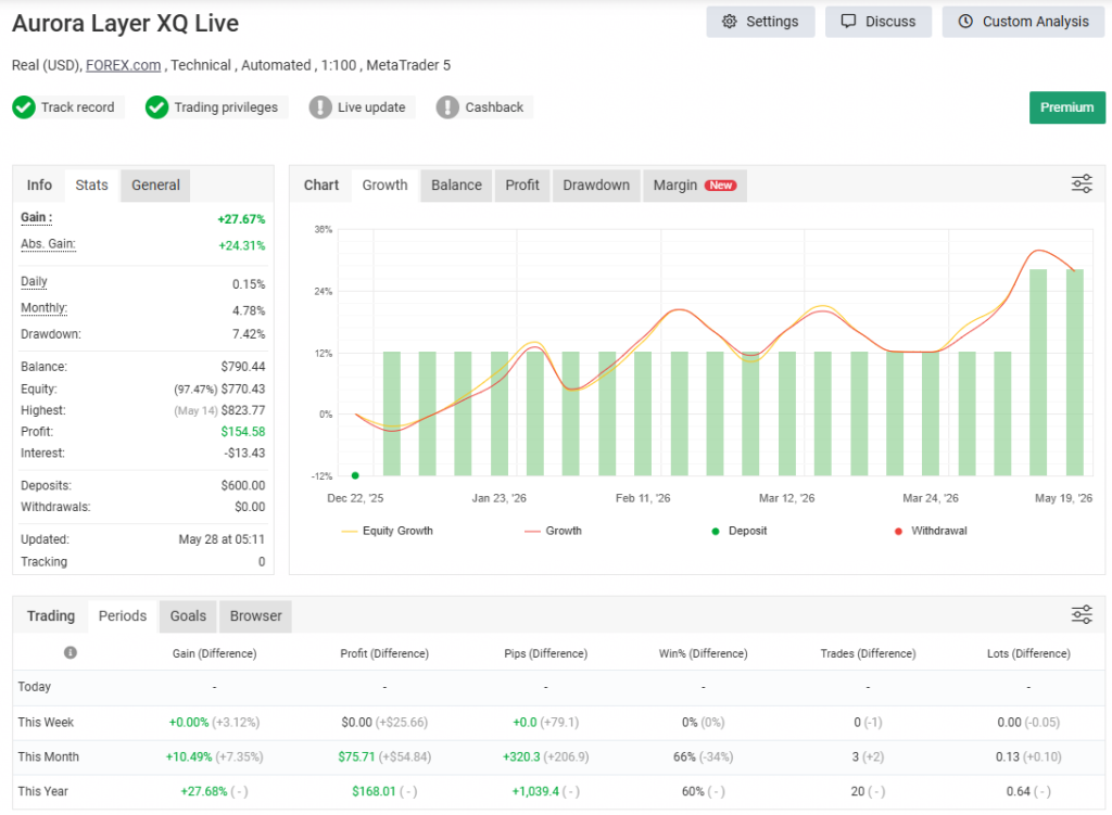
Here is the honest read, and it is the whole lesson of this article. The win rate held up — it actually improved slightly, from 56% to 60%. But the Sharpe ratio collapsed, from 1.42 in the backtest to 0.33 live. Risk-adjusted quality is the first thing to degrade when a strategy meets the real market, and it degrades long before the win rate does. A beginner staring only at the win rate would conclude the system is performing better than the backtest. The Sharpe tells the truer story: the live returns are choppier per unit of risk than the simulation suggested.
Why the gap? Three concrete reasons, none of them mysterious. First, sample size: twenty trades is statistical noise. A Sharpe computed over five months and twenty trades is wildly unstable, whereas the backtest’s figure rests on 305 trades across four years and several market regimes. The live number has not had time to converge. Second, friction the simulator underweights: my live account has paid −$8.96 in commissions and −$13.43 in swap so far, and real USDJPY execution carries spread and slippage during Tokyo and London news spikes that even a real-tick backtest does not fully reproduce. Third, regime luck: the backtest’s fat winners came largely from the 2022–2024 trending yen moves; the live window has been comparatively range-bound, so the average win has been smaller relative to its volatility.
I expected this gap, which is exactly why I report it. A live Sharpe of 0.33 on twenty trades is not a failure — it is an immature sample of a strategy whose underlying edge (profit factor still 1.87, drawdown still contained at 7.42%, below the backtest’s 12.46%) remains intact. The mistake would have been to assume the 1.42 backtest Sharpe would simply reappear live. It never does.
3. Forcing in Market Reality: Friction Costs
A paper profit is a fantasy. In a raw backtest, liquidity is infinite and trades are free. In the real world, every execution incurs friction:
- Exchange/broker fees: Binance, Bybit, and most forex brokers take a commission or spread on both entry and exit. My live commissions above are small in dollars but real, and they compound across hundreds of trades.
- Slippage: the difference between the price your algorithm assumes and the price the order book actually gives you. In fast markets this alone can vaporize a large chunk of theoretical yield.
You must mathematically force these penalties onto the strategy before you believe it. If it cannot survive simulated friction, it does not deserve live capital:
python
import vectorbt as vbt

price = vbt.YFData.download("BTC-USD", start="2022-01-01", end="2026-01-01").get('Close')

fast_ma = vbt.MA.run(price, window=10)
slow_ma = vbt.MA.run(price, window=50)

entries = fast_ma.ma_crossed_above(slow_ma)
exits = fast_ma.ma_crossed_below(slow_ma)

# Instantiate with realistic friction
pf = vbt.Portfolio.from_signals(
    price, entries, exits,
    init_cash=10000,
    fees=0.001,       # 0.1% fee on every buy and sell
    slippage=0.0015,  # 0.15% slippage penalty on execution price
)

print(f"Friction-adjusted return: {pf.total_return() * 100:.2f}%")
For why I moved to VectorBT over event-driven loops when optimizing minute-level data, see my write-up on the Python libraries I actually use for algorithmic trading.
4. The Institutional Standard: Walk-Forward Analysis
Amateurs optimize one giant block of history until it fits perfectly. Professionals use Walk-Forward Analysis: train and optimize on one window, lock those parameters, then test on unseen data, then roll the window forward and repeat. It is the only way to prove a strategy has genuine predictive power rather than excellent historical memory.
I want to be transparent about where Aurora Layer XQ stands on this: the four-year run above is a single in-sample backtest. It is a strong start, but it is not yet walk-forward validated, and I will not pretend otherwise. The discipline I hold myself to is simple — optimize on one window, then freeze the parameters and judge them only on the unseen window that follows; a strategy that needs re-tuning between windows just to stay profitable has no real edge, only a good memory. That rolling validation is the next step I am running for this system, and clearing it is the bar I have set before I would ever scale the position size. One early sign is encouraging but far from conclusive: the live drawdown so far (7.42%) has stayed well inside the envelope the in-sample backtest predicted (12.46% maximal) rather than blowing past it.
5. The Metrics That Actually Matter
Total net profit is a vanity metric — it is the number that sells trading courses and ruins beginners. To judge whether an algorithm is robust enough to deploy, look at its risk profile:
- Maximum Drawdown (MDD): the largest peak-to-trough decline. Can you survive — financially and psychologically — your automated account dropping double digits before it recovers? Mine ran 12.46% in backtest, 7.42% live so far.
- Sharpe Ratio: risk-adjusted return. Above ~1.5 in a fully friction-loaded backtest is generally robust; my backtest landed at 1.42, and watching the live figure converge from its current 0.33 is now the single most important thing I track.
- Profit Factor: gross profit divided by gross loss. Above 1.5 is healthy; 2.17 backtest and 1.87 live both clear it.
- Calmar Ratio: annualized return divided by max drawdown — a great read on how smoothly the system recovers from inevitable losing streaks.
Conclusion
Backtesting is where theory crashes into mathematical reality. By aggressively modeling friction, destroying overfitting, and analyzing drawdown and Sharpe instead of headline returns, you move from retail gambler to quantitative engineer. I learned the hard way that a 1.42 backtest Sharpe does not reappear live on a small sample — and reporting that honestly, with a public track record anyone can audit, is the whole point of doing this in the open.
If you want the production version of this discipline already packaged into a deployable MT5 system — the same Aurora Layer XQ strategy and risk model documented above — that is exactly what the EA is: Aurora Layer XQ on Gumroad.
In the next session we will cover data visualization — plotting these metrics to read the behavioral psychology of an algorithm. Until then: a failed backtest is a cheap lesson compared to a liquidated live account.