
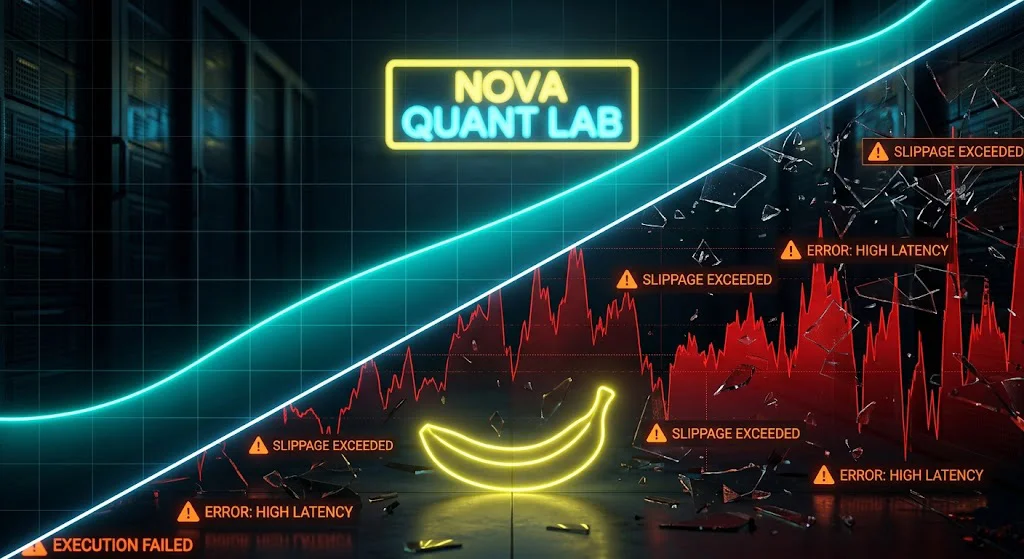
If you have spent any significant amount of time in the quantitative trading space, you have inevitably experienced the most crushing phenomenon in algorithmic development. You spend weeks coding a Python trading algorithm. You run it through your backtesting engine. The equity curve is a perfect, smooth 45-degree angle upward. The Sharpe ratio is above 2.0. The maximum drawdown is a negligible 4%.
Convinced you have found an undeniable edge, you fund a live broker account, deploy the script to your cloud VPS, and wait. Within three weeks, the algorithm is bleeding capital. The entries are late, the exits are inefficient, and that 4% historical drawdown is rapidly approaching 15%.
You are left staring at your terminal, typing a desperate question into Google: “Why do my algorithmic strategies work in backtests but lose money when deployed live?”
You are not alone. This is the universal initiation rite for retail quantitative traders. The brutal reality is that a backtest is not a simulation of the market; it is a simulation of your code running against dead, static numbers. The live market is a living, breathing ecosystem designed to extract liquidity from poorly constructed execution logic.
In this comprehensive guide, we are going to dissect exactly why algorithmic trading strategies fail in live markets. We will break down the mathematical illusions of backtesting, expose the silent killers of algorithmic profitability, and outline the exact protocols required to bridge the gap between historical simulation and live execution.
The Illusion of Infinite Liquidity and Zero Slippage
The single most common reason a profitable backtest turns into a live-market disaster is the misunderstanding of market impact and slippage.
When you build a basic backtest in Python using libraries like pandas or Backtrader, the engine assumes that when your algorithm generates a “BUY” signal at $65,000, you are instantly filled at exactly $65,000. It assumes infinite liquidity.
The Market Order Trap
In the live market, if your algorithm fires a Market Order to buy 1 Bitcoin, you are not buying it at the current mid-price. You are buying it at the best available Ask price. If the order book is thin, your 1 BTC order might eat through three different price levels. You might get 0.2 BTC at $65,000, 0.5 BTC at $65,005, and 0.3 BTC at $65,010. Your average fill price is now significantly worse than your backtest assumed.
This difference between the expected price of a trade and the actual executed price is Slippage.
If your strategy is a high-frequency trading (HFT) bot or a scalper attempting to capture tiny 0.1% price movements, slippage will mathematically destroy your edge. A backtest might show a strategy making 100 trades a day with an average profit of $5 per trade. But if you suffer just $6 of slippage per trade in the live market, your “holy grail” algorithm is actually losing $100 a day.
Spread Widening During Illiquid Hours
If you are trading Forex via MT5, you must also account for variable spreads. Many novice developers use “fixed spread” settings in the MT5 Strategy Tester. This is a fatal error.
During the Asian session crossover or major news events (like NFP or FOMC), liquidity providers pull their orders, and brokers widen their spreads massively to protect themselves. A EUR/USD spread that is normally 0.8 pips can instantly blow out to 15 pips. If your Python or MQL5 bot executes a trade during this window, you start the trade in a massive hole. Your backtest, running on static 1-minute close data, is completely blind to this intra-minute spread widening.
The Fix: You must hardcode pessimistic slippage and dynamic commission models into your backtesting engine. If you are using Python, you should deduct a fixed percentage (e.g., 0.05% for Crypto, 1 pip for Forex) from every single simulated execution. If the strategy’s equity curve collapses after adding realistic slippage, the strategy never had an edge to begin with. It was simply curve-fitted to the illusion of perfect execution.
Look-Ahead Bias: The Silent Assassin in Python
If your backtest shows an astronomically high win rate (above 85%), you have not cracked the market code. You have a bug in your Python script. specifically, you are suffering from Look-Ahead Bias.
Look-ahead bias occurs when your algorithm uses information in the backtest that would have been impossible to know at that exact moment in live trading. It is the equivalent of betting on a horse race after reading tomorrow’s newspaper.
This happens incredibly easily when manipulating Pandas DataFrames for feature engineering. Let’s look at a classic mistake:
Python
import pandas as pd
import numpy as np

# A FATAL FLAW IN FEATURE ENGINEERING
df['Next_Close'] = df['Close'].shift(-1)
df['Signal'] = np.where(df['Next_Close'] > df['Close'], 1, -1)
In the snippet above, the developer shifts the close price backward to create a signal. The backtester executes a trade today based on the knowledge of tomorrow’s closing price. In a backtest, this produces a vertical equity curve. In live deployment, the shift(-1) function evaluates to NaN (Not a Number) because tomorrow’s data does not exist yet. The bot either crashes or trades randomly.
The “End-of-Bar” Execution Trap
Even without blatant coding errors, a subtle form of look-ahead bias plagues moving average crossover strategies.
Let’s assume your logic dictates: “If the 1-hour close price crosses above the 50-SMA, buy.” In a backtest, the engine looks at the 10:00 AM candle, sees it closed above the SMA, and records a buy at the 10:00 AM closing price. However, in live trading, you cannot execute at the 10:00 AM close price after knowing the candle has closed. By the time your Python loop confirms the candle has closed, it is now 10:00:01 AM, and the market has already moved. You are entering the trade on the open of the 11:00 AM candle, which could be drastically different due to a sudden spike.
The Fix: Always offset your signals. If a signal is generated on Candle $T$, your backtester must execute the trade at the Open price of Candle $T+1$. Never assume you can execute at the exact closing price of the candle that generates the signal.
The Curse of Overfitting and Curve Fitting
When we discuss why trading algorithms keep failing in live markets after successful backtesting, we have to address human psychology. When a developer runs a backtest and it loses money, the immediate reaction is not to discard the strategy, but to “tweak the parameters.”
If the 50-period moving average loses money, they test the 55-period. If the RSI threshold of 30 triggers false signals, they change it to 28. They continue optimizing the Take Profit and Stop Loss variables until the equity curve looks perfect.
This is Curve Fitting. You are not discovering a fundamental mathematical truth about market behavior; you are simply creating an algorithm that perfectly memorizes historical noise.
Financial data is largely stochastic (random). When you over-optimize parameters, your Python bot is essentially memorizing exactly what happened in the market between January 2023 and December 2024. But the market regime in 2026 will not behave exactly like 2024. The moment you deploy an overfitted bot into a new, unseen market regime, it breaks down completely because it doesn’t know how to handle variance.
Enter Marcos Lopez de Prado and Purged Cross-Validation
To truly test if a strategy has robustness, we must look to institutional methodologies. In his groundbreaking work on financial machine learning, Marcos Lopez de Prado highlights a critical flaw in standard machine learning cross-validation when applied to finance.
If you use standard K-Fold cross-validation on time-series data, you leak information. Because financial data points are highly serially correlated (today’s volatility is related to yesterday’s), training your model on random chunks of data causes data leakage.
The institutional solution is Purged K-Fold Cross-Validation with Embargoing.
When dividing your historical data into training and testing sets, you must “purge” (delete) a chunk of data right before the testing set, and “embargo” (quarantine) a chunk of data right after. This ensures that the machine learning algorithm or optimization engine cannot use overlapping events to cheat on the test. If your LightGBM model or moving average parameters can survive a strict Purged K-Fold backtest without the equity curve collapsing, you have likely found a genuine, robust edge rather than a curve-fitted illusion.
The Infrastructure Reality: Latency and Execution Bottlenecks
In our previous guides regarding the ultimate 2026 VPS infrastructure, we discussed the absolute necessity of server selection. Backtests do not experience ping latency. Live algorithms do.
Suppose you are running a multi-exchange arbitrage strategy in Python. Your script detects a $15 price discrepancy between Binance and Bybit.
- The backtest assumes instant execution on both legs, locking in $15 of risk-free profit.
- In the live market, your Python script running on a slow, shared web host in Ohio takes 150 milliseconds to send the order to the Tokyo matching engine.
- High-frequency institutional algorithms colocated in Tokyo detect the same discrepancy and execute in 2 milliseconds.
- By the time your order arrives, the liquidity is gone. Your first leg fills, your second leg fails, and you are left holding a naked, unhedged position as the market crashes.
This is why your algorithmic trading strategies keep failing in live markets. You are bringing a knife to a gunfight.
The Fix: Your execution environment must match your backtesting assumptions. If your strategy requires millisecond precision, you cannot run it from your local laptop over Wi-Fi. You must deploy your Python execution engine on a low-latency Linux VPS (like Vultr or DigitalOcean) geographically located as close to the exchange’s matching engine as possible. If you are trading Forex, you need a high-stability Windows VPS (like Hyonix) placed in London or New York to maintain a sub-5ms ping to the MT5 broker servers.
The Paradigm of “Live Forward Testing”
The transition from a backtest to a live, full-capital deployment should never be instantaneous. The gap between history and reality is too vast. The professional protocol to bridge this gap is Live Forward Testing (often called Paper Trading or Incubation).
Once a strategy survives realistic slippage modeling, avoids look-ahead bias, and passes Purged K-Fold cross-validation, it earns the right to be deployed on a demo account or a live account with absolute minimum position sizing (e.g., $10 risk per trade).
During this incubation phase, which should last a minimum of 30 to 60 days, you are not trying to make money. You are collecting data. You are comparing the Live Execution Log against the Backtest Log for the exact same time period.
You must ask yourself:
- Did the backtest generate a trade at 14:00 that the live bot missed? Why? (API timeout? WebSocket disconnect?)
- Did the live bot suffer 3 pips of slippage while the backtest assumed 0?
- Is the Live PnL tracking within a 10% margin of error compared to the Backtest PnL?
Only when the live, forward-tested equity curve mathematically correlates with the simulated backtest curve do you slowly begin scaling up your position sizing.
The Bottom Line for 2026
The reason your trading algorithms keep failing in live markets after successful backtesting is that a backtester is inherently optimistic, while the live market is inherently predatory.
A backtest is merely the first step in a very long scientific process. It is a tool for disproving bad ideas, not validating good ones. If a strategy fails a backtest, throw it away. If it passes a backtest, you have simply earned the right to begin the real work: modeling slippage, eliminating look-ahead bias, punishing the parameters with out-of-sample data, and deploying it into a heavily monitored, low-latency forward testing environment.
Stop treating your backtest equity curve as a prophecy. Treat it as a hypothesis. Prove it in the live fire of the market before you trust it with your capital.